
Deep-learning-based MRI in the diagnosis of cerebral infarction and its correlation with the neutrophil to lymphocyte ratio
Introduction
In addition to being the most common and frequently occurring disease in clinical settings, the incidence of vertigo disease is increasing every year. Patients who complain of vertigo account for about 5% of the patients of the Internal Medicine Department, and 15% of the patients of the Otolaryngology Department. The disease is more common in the elderly (1,2). At present, research on vertigo disease is limited, and vertigo is the only major symptom of the disease. The main causes of vertigo disease are organic and functional lesions (3).
Due to rapid advances, imaging technology now plays a crucial role in the diagnosis of vertigo disease. The occurrence of cardiovascular and cerebrovascular diseases for which vertigo is the chief complaint can now be effectively prevented by the quantitative analysis of medical images (4). In the early diagnosis of disease, image segmentation technology can help doctors to distinguish between normal and pathological tissue more precisely, and make full use of detailed information about lesion areas for the diagnosis and treatment of diseases (5). Traditional image segmentation algorithms are composed of segmentations, such as edge-based segmentation and area segmentation. However, as traditional image segmentation algorithms can only use information on the gray scale of an image to segment the target area and lack spatial information, such algorithms are more sensitive to noise in images (6,7). With the emergence and growth of deep learning (DL), new segmentation technology has achieved excellent results in terms of computer-vision tasks.
In recent years, many studies have confirmed that the neutrophil to lymphocyte ratio (NLR) is closely correlated to the prognosis of patients with atherosclerosis, malignant tumors, and severe pancreatitis (8). To explore the application effects of DL technology in the segmentation and processing of magnetic resonance imaging (MRI) of the brains of patients, and the efficiency of the NLR and other routine blood indexes in the diagnosis of vertiginous cerebral infarction (VCI), DL technology for the segmentation of MRI of patients’ brains was first constructed. The effects of the NLR and other indexes in the diagnosis of VCI were compared and analyzed based on the gold standard for VCI patients (i.e., diagnosis results). This research sought to raise the diagnostic efficiency of VCI in clinical practice. We present the following article in accordance with the STARD reporting checklist (available at https://dx.doi.org/10.21037/apm-21-1786).
Methods
Convolutional neural network (CNN)
The CNN is a category of DL methods, which has been applied in image segmentation and early phase processing. Its basic structure mainly comprises an input layer, hidden layer, and output layer. The hidden layer usually consists of convolutional, pooling and fully connected layers (9) (see Figure 1).
Convolutional layer
A convolution is a mathematical operator used to generate a 3rd function by virtue of 2 functions. Provided that f (x) and g (x) are integrable functions and the convolutional operation is defined as *, the function h (x) is calculated as follows:
In Eq. [1], the h (x) function is also an integrable function.
The convolution kernel in a CNN is composed of a weight matrix. The convolution operation is the process by which the feature graphs pass through the moving filters of the convolution kernel. When the filter skims over the relevant position in an image, the multiplying and summing process is deemed as the discretization of the above integrations, and the mathematical equation is expressed as follows:
where f (x, y) represents the gray scale value of the pixels at (x, y) location in images, ω (u, v) represents the weighted value at the (u, v) location of the weight matrix, both a and b are positive integers, (·) is a product sum of the weight matrix and its image pixels around, β represents the bias, and λ represents the activation function.
Pooling layer
The pooling layer (also referred to as the sampling layer) is usually used alternately with the convolutional layer. It is mainly applied in the dimensional reduction of the output feature graphs in the preceding convolution layer to cut down the size of the feature graphs. The pooling operation can be considered a special operation of the moving filter. Common pooling operations serve as mean-pooling and max-pooling methods (10). The mean-pooling operation returns to the range of the moving window, which is referred to as the mean value. The max-pooling operation returns to the range of the moving window, which is referred to as the maximum value. The latter ensures no change to the features in the feature graphs; thus, it is generally used in CNN. The moving window in the pooling layer usually has a size of 2×2 and a step length of 2.
Fully connected layer
When a CNN model is applied in image classification, the fully connected layer is usually located at the end of the model to connect the output layer of the model (see Figure 1). The fully connected layer is mainly applied in the classification and processing of data and images. The mathematical equation is expressed as follows:
where xi represents the input value of i nerve cells, ωi indicates the connection value of i nerve cells and current nerve cells, and θ is the threshold of the current nerve.
The output layer in the CNN model is generally composed of “N” nerve cells with an identical number of categories that are to be classified. When the nerve cells in the output layer of the model deliver the results, it is required to obtain a 1-dimensional (1D) vector with a length of N through the Softmax function. The 1D vector represents the probability that the input image belongs to a certain category.
Activation function
The activation function is a critical step in the network model, and can directly determine the state of nerve cells in the model. The activation function can be classified into functions such as the Sigmoid, Tanh, and Rectified Linear Unit (ReLU) functions (11). The Sigmoid function is able to map the images to the (0, 1) range. The mathematical equation for the activation function is expressed as follows:
In the back propagation algorithm, when the derivation of the activation function is required, the derivative of the Sigmoid activation function with respect to “x” can be represented by the function itself, which is as follows:
The Sigmoid function is an increasing activation function with a simple derivation process. Thus, it is frequently used in the loss function in the neural network model. The Sigmoid function in reverse propagation is prone to small gradient, but it is not applicable to the training of a deep network. The Tanh function is similar to the Sigmoid function. The mathematical equation for the Tanh function is expressed as follows:
The Tanh function can also map the input image to the (0, 1) range to obtain the mean value with the output of 0. In actual application, the training effect of the Tanh activation function is superior to that of the Sigmoid function; however, the Tanh activation function also carries the risk of the gradient vanishing. Thus, the ReLU activation function used in the AlexNet model can address the weakness of the Sigmoid and Tanh functions. The mathematical equation for the ReLU is expressed as follows:
U-type full convolutional network (FCN)
The FCN has higher segmentation accuracy than the CNN model; however, it has a more complicated training process, and is less precise in the segmentation of details in images (12). The U-type convolutional network (U-Net) was improved based on the FCN model and is mainly made up of 2 U-shape structures (see Figure 2).
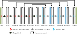
The contraction path is located on the left side. First, two successive convolutional layers are used. Next, the max-pooling layer with a step length of 2 is used to down sample the feature graphs (the operation is repeatedly performed 4 times). The expansion path is located on the right side. First, the results output from the contraction path undergo the down-sampling operation. Next, the size of the feature graphs is returned to the original size using two successive convolutional layers (the operation is repeatedly performed 4 times). The jump connection is also used in the network. This operation can transmit the feature graphs from the shallow layer to the high layer efficiently to obtain information about the features with different dimensions. The ReLU function serves as the activation function in the model.
Experimental materials
Research subjects
A total of 115 VCI patients (83 male and 32 female), admitted to the Department of Neurology at Huizhou Central People’s Hospital from January 2016 to December 2020, were chosen as the research subjects. All of the patients reported experiencing different degrees of dizziness. The ages of the patients ranged from 31 to 88 years old, and the patients had an average age of 63.28±10.16 years old. All procedures performed in this study involving human participants were in accordance with the Declaration of Helsinki (as revised in 2013). The study was approved by ethics board of Huizhou Central People’s Hospital (No. kyll2021223) and informed consent was taken from all the patients.
Inclusion and exclusion standard
To be eligible to participate in the study, patients had to meet the following inclusion standard: (I) have vertigo symptoms, including dizziness, blurred vision, nausea, nystagmus, tinnitus, deafness, and ataxia; and (II) have undergone MRI diagnoses and have complete clinical data. Participants were excluded from the study if they met any of the following exclusion criteria: (I) had vertigo disease arising from Meniere disease, labyrinthitis, or trauma; (II) had suffered from a severely infectious disease, tumor, or severe liver or renal disease; (III) had received incomplete clinical treatment; and/or (IV) had been diagnosed with encephalorrhagia via MRI.
Experimental method
MRI examination
All the patients underwent MRI (or Diffusion-Weighted Imaging, DWI) examinations. The Signa Exlicte3.0T MRI machine of GE was used to collect images of the patients’ brains. The MRI acquisition covered T1- fluid attenuated inversion recovery (FLAIR), T2-fast spin echo (FSE), and T2-FLAIR sequences for set scanning parameters (see Table 1). In addition, the parameters of the intracranial scan for the anterior and posterior circulation of the patient included the layer thickness (1.0 mm), flip angle (20°), visual field (18 cm), and matrix (512×256).
Table 1
| Sequence | Position | TR (ms) | TE (ms) | TI (ms) |
|---|---|---|---|---|
| T1-FLAIR | Sagittal view | 1,750 | 8.9 | 920 |
| Axial view | 3,196 | 7.9 | 960 | |
| T2-FLAIR | Axial view | 10,002 | 115 | 2,300 |
| T2-FSE | Axial view | 5,100 | 118 | – |
MRI, magnetic resonance imaging; FLAIR, fluid attenuated inversion recovery; FSE, fast-spin echo; TR, repetition time; TE, echo time; TI, inversion time.
MRI segmentation based on the MS (U-Net) model
The U-Net model could not precisely segment the MRI of the brain. Thus, we introduced the inception model based on the U-Net model and constructed a multiscale U-Net [MS (U-Net)] model. The MS (U-Net) model had a convolutional layer for which the convolution kernel sizes of 1×1 and 5×5 were based on the U-Net model. The complete structure of the MS (U-Net) model is shown in Figure 3.
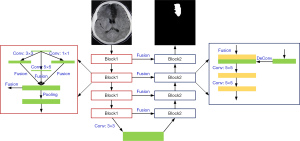
The convolution kernel sizes of 1×1, 3×3, and 5×5 were entered into the Block 1 module of the MS (U-Net) model for image convolutional processing to obtain three kinds of feature graphs with different sizes and the same contents; three kinds of feature graphs were combined in the fusion layer. The size of the feature graphs was dwindled using the pooling layer, and delivered to the next module (the step was repeatedly performed 4 times). The deconvolution of the input feature graphs was performed, and the processed results and the output results of the Block 1 module (Block 1 and Block 2 were connected) were integrated. The convolution layer was used to perform the convolution operation for fusion results, and transmit them to the next module (the step was repeatedly performed 4 times). Finally, 4 convolutional layers with the convolution kernels size of 1×1 were used to process the last Block 2 module, and the segmentation graphs were classified using the Softmax.
1,800 brain MR images with a size of 256×256 were used to train the model. MRI of the brain were segmented into gray matter (GM), white matter (WM), cerebrospinal fluid (CSF), and background (BG) using the model. Cross-entropy was employed as the loss function, the training optimization process served as the Adam function, and the initial learning rate was set as 0.0001 in the models constructed in this study.
Data collection
In accordance with the patient record system and related examinations at the hospital, general information about each patient (i.e., age, gender and past medical history, including details of hypertension, diabetes, coronary heart disease, smoking and alcohol abuse) was collected. The patient started fasting on the 2nd day after admission to the hospital. After 8–12 hours, 5 mL of venous blood was collected from each patient in the supine position. The blood cells and blood biochemical indexes were tested with an automatic biochemical analyzer. The neutrophil, lymphocyte, high-density lipoprotein (HDL), and low-density lipoprotein (LDL) were detected to calculate the NLR.
Statistical analysis
The SPSS22.0 software package was used in the statistical analysis. The measurement data that conformed to the normal distribution are presented as the mean value ± standard deviation, while the measurement data that did not conform to the normal distribution are presented as the median and quartiles. The enumeration data are presented as the number of cases and percentage [n (%)]. The measurement data were verified by independent sample t and sum of ranks tests, while the enumeration data were verified by chi-square and sum of ranks tests. The MRI diagnosis served as the gold standard. The receiver operating characteristic (ROC) curve was drawn to analyze the diagnosis effect. A P<0.05 indicated a statistically significant difference.
Results
Evaluation of MRI segmentation results for images of MS (U-Net) models
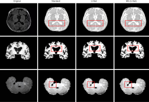
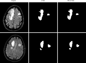
The MS (U-Net) model and the original U-Net model were compared to examine the segmentation effects of MRI of the brain (see Figure 4). The segmentation results of the MS (U-Net) model were closer to the standard segmentation results than those of the U-Net model. Additionally, the MS (U-Net) model retains the details of CSF in the MRI and highly restores the segmentation effect of CSF around the GM after segmentation. The MS (U-Net) model segmentation results showed that there was a more delicate border between the alba and GM. In short, the MS (U-Net) model constructed in this study that was applied in the segmentation of MRI of the brain was better able to process details than the original U-Net model, and its results were much closer to the real segmentation results.
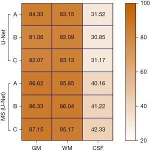
To assess the segmentation effects of MRI of the brain of different models quantitatively, Jaccard similarity (Js) was used as the evaluation indicator. The higher the Js value, the more accurate the segmentation effect of the model. The calculation equation of the Js value is expressed as follows:
where M represents the segmentation results of the model, and S indicates the standard segmentation results.
The GM, WM, and CSF in three different MRI images of the brain of the U-Net model and MS (U-Net) model were analyzed to examine differences in their Js values (see Figure 5). The results showed that the Js values for GM and WM in the U-Net model and MS (U-Net) model were higher than 80%, and the segmented Js value of the MS (U-Net) model was higher than that of the U-Net model. The CSF-segmented Js values of the U-Net model and MS (U-Net) model were quite low. In general, the MS (U-Net) had a higher segmented Js value, which indicated that the MS (U-Net) model proposed in the study was more stable than the U-Net model in the segmentation of MRI of the brain.
Segmentation of MRI for vertigo patients based on the MS (U-Net) model
The U-Net model and MS (U-Net) model were used to segment MRI of the brains of the vertigo patients in the study (see Figure 6). The MS (U-Net) model proposed in the article was able to segment the lesion locations in the MRI of the patients more precisely than the U-Net model.
Comparison of clinical data of patients
Fifty healthy individuals, who received a physical examination at our hospital during the same period, were allocated to the control group. According to the MRI diagnosis results, 115 vertigo patients were allocated to the benign paroxysmal positional vertigo (BPPV) group (n=70) or the acute cerebral infarct (ACI) group (n=45). First, differences in the clinical data of patients were compared (see Table 2). There was no apparent difference among the control group, BPPV group and ACI group in terms of age and gender (P>0.05). The proportion of patients with a history of smoking, alcohol abuse, diabetes, and coronary heart disease in the BPPV group and ACI group was higher than that of the control group (P<0.05). Additionally, the proportion of patients with a history of hypertension in the ACI group was high (P<0.05), and the proportion of patients with a history of smoking, hypertension, and diabetes was significantly higher in the in the ACI group than the BPPV group (P<0.05).
Table 2
| Information | Control group (n=50) | BPPV group (n=70) | ACI group (n=45) |
|---|---|---|---|
| Age (years old) | 60.86±10.26 | 61.88±12.15 | 62.07±11.38 |
| Male (case/%) | 37/74.00 | 52/74.29 | 31/68.89 |
| Smoking history (case/%) | 12/24.00 | 23/32.86* | 22/48.89*# |
| Alcohol abuse (case/%) | 10/20.00 | 21/30.00* | 14/31.11* |
| Hypertension (case/%) | 26/52.00 | 38/54.29 | 30/66.67*# |
| Diabetes (case/%) | 9/18.00 | 15/21.43* | 12/26.67*# |
| Coronary heart disease (case/%) | 4/8.00 | 9/12.86* | 5/11.11* |
As compared to the control group, *P<0.05; as compared to the BPPV group, #P<0.05. BPPV, benign paroxysmal positional vertigo; ACI, acute cerebral infarct.
Comparison of routine blood examination results of patients
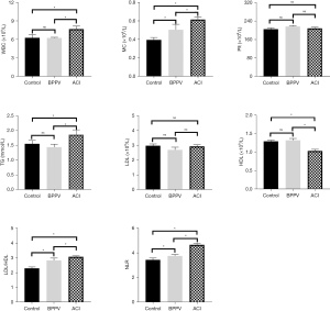
Figure 7 shows the difference in the routine blood examination results of all groups of patients. The monocyte count (MC), LDL/HDL ratio, and NLR of patients in the BPPV group were higher than those of patients in the control group (P<0.05). Compared with the control group, the levels of WBC, TG, MC, LDL/HDL and MLR in ACI patients were significantly increased (P<0.05), and the levels of HDL were significantly decreased (P<0.05). Compared with the BPPV group, the levels of WBC, MC, TG, LDL/HDL and NLR in ACI patients were significantly increased (P<0.05), while the levels of HDL were significantly decreased (P<0.05). The patients in the control group and BPPV group showed no obvious differences in terms of their WBCs, TG and HDL levels (P>0.05); all groups of patients showed no difference in terms of the platelet counts and LDL levels (P>0.05).
Comparison of diagnostic efficiency of indicators
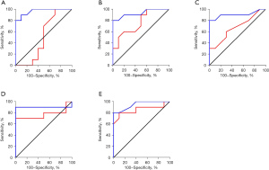
The ROC curves were outlined to analyze the different routine blood indexes, and determine the diagnostic efficiency for the BPPV and ACI patient groups (see Figure 8). The AUCs of the WBC, TG level, HDL level, LDL/HDL ratio, and NLR of the ACI patients were 0.965, 0.930, 0.905, 0.900, and 0.945, respectively, showing obvious differences in diagnosing BPPV and ACI (P=0.000, 0.001, 0.002, 0.003, and 0.001). The AUCs of the TG level, LDL/HDL ratio, and the NLR of BPPV patients were 0.760, 0.770, and 0.855, respectively, showing obvious differences in diagnosing BPPV and ACI (P=0.049,0.041,0.007). However, the AUCs of the WBC and HDL level of the BPPV patients were 0.500 and 0.670, respectively, showing obvious differences in diagnosing BPPV and ACI (P=0.999, 0.199).
Discussion
The incidence of vertigo may be caused by vertebrobasilar artery lesions, vestibular blood supply insufficiency, and ischemic stroke (13). The diseases with vertigo as the main complaint have attracted widespread attention because the patients are increasingly younger. MRI technology continues to have excellent application value in the early diagnosis of cerebrovascular diseases, and can cure vertigo disease caused by vascular lesions (14).
DL technology has been applied in MRI-aided diagnoses of patients, and has been shown to dramatically improve the diagnosis efficiency of the disease (15). The traditional CNN model is mainly applied in the classification and processing of images. The FCN has been used to address the lengthy training time issue and other issues in the image segmentation. The U-Net model has poor detail segmentation effects in terms of the segmentation and processing of MRI of the brain (16-18). Based on the U-Net model, the concept of a multiscale model was introduced, and a MS U-Net model was constructed in this study. This MS U-Net model was applied in MRI segmentation. We found that the MS U-Net model had higher segmentation precision than the U-Net model, and its segmentation results were closer to the standard segmentation results than those of the traditional U-Net model.
The MS U-Net model proposed in this study was then used in the segmentation and processing of MRI of the brains of VCI patients, and was found to effectively segment the infarct regions. Cerebral infarction refers to a blood supply disorder of the local brain tissue arising from multiple factors. Studies have shown that if a patient has an acute cerebral infarction (ACI), in vivo neutrophils can preferentially reach the patient’s ischemic area and destroy the blood-brain barrier by releasing proteolytic enzyme, which interacts with platelets to aggravate brain damage (19,20).
The WBC is the most common clinical index for evaluating the inflammatory response of the human body (21). Many studies have confirmed that monocytes and HDL are closely correlated with the occurrence and progression of atherosclerosis and other cardiovascular and cerebrovascular diseases (22,23). In this study, DL-based MRI was used to analyze diagnoses of BPPV and ACI, and compare differences between BPPV patients and ACI patients in terms of the WBC, platelet count, HDL, LDL, and TG levels, the LDL/HDL ratio, the NLR, and other indicators. The results showed that compared to BPPV patients, the WBC, MC, TG level, LDL/HDL ratio, and NLR of ACI patients increased significantly (P<0.05), while their HDL level decreased significantly (P<0.05). Additionally, we showed that the WBC, TG and HDL levels, LDL/HDL ratio and NLR can be applied in the diagnosis of ADI diseases. Thus, these indicators can serve as auxiliary diagnostic indicators for ACI patients with vertigo symptoms.
Conclusions
In conclusion, DL technology was applied in the segmentation and processing of MRI of the brains of the VCI patients to obtain better segmentation results of lesion areas. The WBC, TG level, HDL level, LDL/HDL ratio, NLR, and other indexes reflect the VCI severity of patients to some extent. However, it should be noted that this study had some limitations. Notably, only differences in the clinical routine blood indexes of BPPV patients and ACI patients were analyzed; however, the question of whether all the indexes can serve as independent predictors in VCI diagnosis was not explored. The study also had a very limited sample size, which should be increased in future clinical observations and investigations.
Acknowledgments
Funding: None.
Footnote
Reporting Checklist: The authors have completed the STARD reporting checklist. Available at https://dx.doi.org/10.21037/apm-21-1786
Data Sharing Statement: Available at https://dx.doi.org/10.21037/apm-21-1786
Conflicts of Interest: All authors have completed the ICMJE uniform disclosure form (available at https://dx.doi.org/10.21037/apm-21-1786). The authors have no conflicts of interest to declare.
Ethical Statement: The authors are accountable for all aspects of the work in ensuring that questions related to the accuracy or integrity of any part of the work are appropriately investigated and resolved. All procedures performed in this study involving human participants were in accordance with the Declaration of Helsinki (as revised in 2013). The study was approved by ethics board of Huizhou Central People’s Hospital (No. kyll2021223) and informed consent was taken from all the patients.
Open Access Statement: This is an Open Access article distributed in accordance with the Creative Commons Attribution-NonCommercial-NoDerivs 4.0 International License (CC BY-NC-ND 4.0), which permits the non-commercial replication and distribution of the article with the strict proviso that no changes or edits are made and the original work is properly cited (including links to both the formal publication through the relevant DOI and the license). See: https://creativecommons.org/licenses/by-nc-nd/4.0/.
References
- Neuhauser HK. The epidemiology of dizziness and vertigo. Handb Clin Neurol 2016;137:67-82. [Crossref] [PubMed]
- Kim HA, Bisdorff A, Bronstein AM, et al. Hemodynamic orthostatic dizziness/vertigo: Diagnostic criteria. J Vestib Res 2019;29:45-56. [Crossref] [PubMed]
- Wipperman J. Dizziness and vertigo. Prim Care 2014;41:115-31. [Crossref] [PubMed]
- Baráth K, Schuknecht B, Naldi AM, et al. Detection and grading of endolymphatic hydrops in Menière disease using MR imaging. AJNR Am J Neuroradiol 2014;35:1387-92. [Crossref] [PubMed]
- Rebelo J, Fernandes K, Cardoso JS. Quality-based Regularization for Iterative Deep Image Segmentation. Annu Int Conf IEEE Eng Med Biol Soc 2019;2019:6734-7. [Crossref] [PubMed]
- Li H, Chen C, Fang S, et al. Brain MR image segmentation using NAMS in pseudo-color. Comput Assist Surg (Abingdon) 2017;22:170-5. [Crossref] [PubMed]
- Flannery SW, Kiapour AM, Edgar DJ, et al. Automated magnetic resonance image segmentation of the anterior cruciate ligament. J Orthop Res 2021;39:831-40. [Crossref] [PubMed]
- Balta S, Celik T, Mikhailidis DP, et al. The Relation Between Atherosclerosis and the Neutrophil-Lymphocyte Ratio. Clin Appl Thromb Hemost 2016;22:405-11. [Crossref] [PubMed]
- Yasaka K, Akai H, Kunimatsu A, et al. Deep learning with convolutional neural network in radiology. Jpn J Radiol 2018;36:257-72. [Crossref] [PubMed]
- Cai T, Zhao Z. Convolutional neural network-based surgical instrument detection. Technol Health Care 2020;28:81-8. [Crossref] [PubMed]
- Anwar SM, Majid M, Qayyum A, et al. Medical Image Analysis using Convolutional Neural Networks: A Review. J Med Syst 2018;42:226. [Crossref] [PubMed]
- Shelhamer E, Long J, Darrell T. Fully Convolutional Networks for Semantic Segmentation. IEEE Trans Pattern Anal Mach Intell 2017;39:640-51. [Crossref] [PubMed]
- Li Y, Peng B. Pathogenesis, Diagnosis, and Treatment of Cervical Vertigo. Pain Physician 2015;18:E583-95. [PubMed]
- Conte G, Lo Russo FM, Calloni SF, et al. MR imaging of endolymphatic hydrops in Ménière's disease: not all that glitters is gold. Acta Otorhinolaryngol Ital 2018;38:369-76. [Crossref] [PubMed]
- Akkus Z, Galimzianova A, Hoogi A, et al. Deep Learning for Brain MRI Segmentation: State of the Art and Future Directions. J Digit Imaging 2017;30:449-59. [Crossref] [PubMed]
- Sarıgül M, Ozyildirim BM, Avci M. Differential convolutional neural network. Neural Netw 2019;116:279-87. [Crossref] [PubMed]
- Ha R, Chang P, Mema E, et al. Fully Automated Convolutional Neural Network Method for Quantification of Breast MRI Fibroglandular Tissue and Background Parenchymal Enhancement. J Digit Imaging 2019;32:141-7. [Crossref] [PubMed]
- Falk T, Mai D, Bensch R, et al. U-Net: deep learning for cell counting, detection, and morphometry. Nat Methods 2019;16:67-70. [Crossref] [PubMed]
- Perez-de-Puig I, Miró-Mur F, Ferrer-Ferrer M, et al. Neutrophil recruitment to the brain in mouse and human ischemic stroke. Acta Neuropathol 2015;129:239-57. [Crossref] [PubMed]
- García-Culebras A, Durán-Laforet V, Peña-Martínez C, et al. Role of TLR4 (Toll-Like Receptor 4) in N1/N2 Neutrophil Programming After Stroke. Stroke 2019;50:2922-32. [Crossref] [PubMed]
- Carisch L, Stirn M, Hatt JM, et al. White blood cell count in birds: evaluation of a commercially available method. BMC Vet Res 2019;15:93. [Crossref] [PubMed]
- Honold L, Nahrendorf M. Resident and Monocyte-Derived Macrophages in Cardiovascular Disease. Circ Res 2018;122:113-27. [Crossref] [PubMed]
- Kornmueller K, Vidakovic I, Prassl R. Artificial High Density Lipoprotein Nanoparticles in Cardiovascular Research. Molecules 2019;24:2829. [Crossref] [PubMed]
(English Language Editor: L. Huleatt)


